41 how to show data labels as percentage in excel
Show Percentages in a Stacked Column Chart in Excel 29 Sept 2018 ... #9 select one data label in the stacked column chart, and then type = in the formula bar, and then select percentage value, and press Enter key. Add or remove data labels in a chart - support.microsoft.com Click Label Options and under Label Contains, select the Values From Cells checkbox. When the Data Label Range dialog box appears, go back to the spreadsheet and select the range for which you want the cell values to display as data labels. When you do that, the selected range will appear in the Data Label Range dialog box. Then click OK.
DataLabels.ShowPercentage property (Excel) | Microsoft Docs Example This example enables the percentage value to be shown for the data labels of the first series on the first chart. This example assumes that a chart exists on the active worksheet. Sub UsePercentage() ActiveSheet.ChartObjects(1).Activate ActiveChart.SeriesCollection(1) _ .DataLabels.ShowPercentage = True End Sub

How to show data labels as percentage in excel
Percent charts in Excel: creation instruction Now we show the percentage of taxes in the diagram. Click the right mouse button. In the dialog box select a task "Add Data Labels". The values from the second column of the table will be on the parts of the circle: Once again right click on the chart and select the item "Format Data Labels": Excel tutorial: How to build a 100% stacked chart with percentages F4 three times will do the job. Now when I copy the formula throughout the table, we get the percentages we need. To add these to the chart, I need select the data labels for each series one at a time, then switch to "value from cells" under label options. Now we have a 100% stacked chart that shows the percentage breakdown in each column. How to create a chart with both percentage and value in Excel? In the Format Data Labels pane, please check Category Name option, and uncheck Value option from the Label Options, and then, you will get all percentages and values are displayed in the chart, see screenshot: 15.
How to show data labels as percentage in excel. Change the format of data labels in a chart To get there, after adding your data labels, select the data label to format, and then click Chart Elements > Data Labels > More Options. To go to the appropriate area, click one of the four icons ( Fill & Line, Effects, Size & Properties ( Layout & Properties in Outlook or Word), or Label Options) shown here. How to add Axis Labels (X & Y) in Excel & Google Sheets Excel offers several different charts and graphs to show your data. In this example, we are going to show a line graph that shows revenue for a company over a five-year period. In the below example, you can see how essential labels are because in this below graph, the user would have trouble understanding the amount of revenue over this period. Excel tutorial: How to use data labels In this video, we'll cover the basics of data labels. Data labels are used to display source data in a chart directly. They normally come from the source data, but they can include other values as well, as we'll see in in a moment. Generally, the easiest way to show data labels to use the chart elements menu. When you check the box, you'll see ... Excel chart to display both values & percentage Re: Excel chart to display both values & percentage. With Chart Type set to Pie, yes you can. Change your chart type to Pie, and right click on the values, pick Format Data Labels and tick Percentage . Register To Reply.
How to show data label in "percentage" instead of - Microsoft Community Select Format Data Labels Select Number in the left column Select Percentage in the popup options In the Format code field set the number of decimal places required and click Add. (Or if the table data in in percentage format then you can select Link to source.) Click OK Regards, OssieMac Report abuse 8 people found this reply helpful · How To Add Data Labels In Excel - lakesidebaptistchurch.info To format data labels in excel, choose the set of data labels to format. Select the chart label you want to change. Read our step by step guide here. Click The Chart To Show The Chart Elements Button. Now that you have an address list in a spreadsheet, you can import it into microsoft word to turn it into labels. Count and Percentage in a Column Chart - ListenData Steps to show Values and Percentage 1. Select values placed in range B3:C6 and Insert a 2D Clustered Column Chart (Go to Insert Tab >> Column >> 2D Clustered Column Chart). See the image below Insert 2D Clustered Column Chart 2. In cell E3, type =C3*1.15 and paste the formula down till E6 Insert a formula 3. Display Data as Percentage of Total in Pivot Table | Microsoft Excel ... 4. A dialog box will appear. Click on the tab Show Value As. 5. Click the drop down menu of Show Values As.In this menu select whatever percentage you want to select. 6. Final result will be like this: You can notice that data is being shown as a percentage of total in your pivot table.
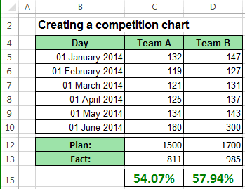
How to Add Percentages to Excel Bar Chart If we would like to add percentages to our bar chart, we would need to have percentages in the table in the first place. We will create a column right to the column points in which we would divide the points of each player with the total points of all players. We will select range A1:C8 and go to Insert >> Charts >> 2-D Column >> Stacked Column ... Percentage Change Chart - Automate Excel Click on Format Data Series . 3. Change Series Overlap to 0%. 4. Change Gap Width to 0% . Your graph should look something like this so far . 5. Select Invisible Bars. 6. Click Format. 7. Select Shape Fill. 8. Click No Fill . Adding Labels. While still clicking the invisible bar, select the + Sign in the top right; Select arrow next to Data ... How To Show Percentages in Stacked Charts (in addition to values) Download the workbook here: the full Excel Dashboard course here: ... How to display percentage labels in pie chart in Excel - YouTube to display percentage labels in pie chart in Excel
Excel Chart Elements: Parts of Charts in Excel | ExcelDemy
Format Data Labels in Excel- Instructions - TeachUcomp, Inc. To format data labels in Excel, choose the set of data labels to format. To do this, click the "Format" tab within the "Chart Tools" contextual tab in the Ribbon. Then select the data labels to format from the "Chart Elements" drop-down in the "Current Selection" button group. Then click the "Format Selection" button that ...

Pie Chart - PK: An Excel Expert
Create Dynamic Chart Data Labels with Slicers - Excel Campus Feb 10, 2016 · Typically a chart will display data labels based on the underlying source data for the chart. In Excel 2013 a new feature called “Value from Cells” was introduced. This feature allows us to specify the a range that we want to use for the labels. Since our data labels will change between a currency ($) and percentage (%) formats, we need a ...
How to Add Data Labels in Excel - Excelchat | Excelchat
Make a Percentage Graph in Excel or Google Sheets Find Percentages. Duplicate the table and create a percentage of total item for each using the formula below (Note: use $ to lock the column reference before copying + pasting the formula across the table). Each total percentage per item should equal 100%. Add Data Labels on Graph. Click on Graph; Select the + Sign; Check Data Labels
Excel Dashboard Templates Friday Challenge Answer - Create a Percentage (%) and Value Label ...
How to Display Percentage in an Excel Graph (3 Methods) Then go to the More Options via the right arrow beside the Data Labels. Select Chart on the Format Data Labels dialog box. Uncheck the Value option. Check the Value From Cells option. Then you have to select cell ranges to extract percentage values. For this purpose, create a column called Percentage using the following formula: =E5/C5
Create stacked column chart with percentage
How to Show Percentage in Pie Chart in Excel? - GeeksforGeeks Jun 29, 2021 · Show percentage in a pie chart: The steps are as follows : Select the pie chart. Right-click on it. A pop-down menu will appear. Click on the Format Data Labels option. The Format Data Labels dialog box will appear. In this dialog box check the “Percentage” button and uncheck the Value button. This will replace the data labels in pie chart ...

E-xcel Tuts: Add Data Labels to Excel Charts
Add Value Label to Pivot Chart Displayed as Percentage Aug 28, 2014. #1. I have created a pivot chart that "Shows Values As" % of Row Total. This chart displays items that are On-Time vs. items that are Late per month. The chart is a 100% stacked bar. I would like to add data labels for the actual value. Example: If the chart displays 25% late and 75% on-time, I would like to display the values ...
Creating a chart with dynamic labels - Microsoft Excel 2013
How To Show Values & Percentages in Excel Pivot Tables Choose Show Value As > % of Grand Total. In some versions of Excel, it might show as % of Total. This is fine. Newer versions of Excel, like Excel 2016, Excel 2019 or Microsoft 365 show a % of Grand Total when you right-click on any numeric value. This is the key way to create a percentage table in Excel Pivots. The Pivot view now changes to this:
Tableau Bar Chart Labels Overlapping - Free Table Bar Chart
How to Show Percentage in Excel Pie Chart (3 Ways) - ExcelDemy Another way of showing percentages in a pie chart is to use the Format Data Labels ...
How-to Put Percentage Labels on Top of a Stacked Column Chart - Excel Dashboard Templates
How to Calculate Price Increase Percentage in Excel (3 Easy Ways) 3 Easy Ways to Calculate Price Increase Percentage in Excel. This article will show the price increment in a percentage format. So, the new price of the products will be greater than the previous one. To illustrate, we'll use a sample dataset as an example. For instance, the following dataset has 4 Products, their Old and New Prices.
Excel Chart Data Labels - Microsoft Community
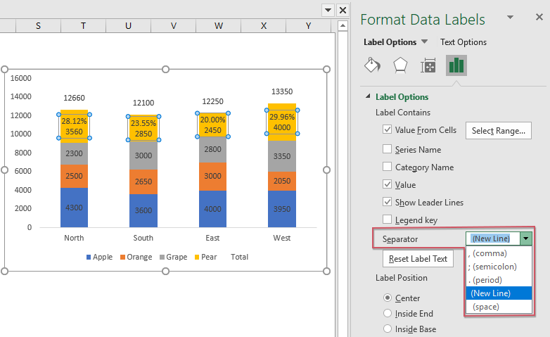
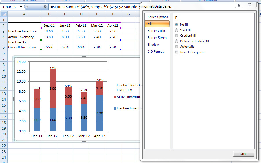
How to Show Percentages in Stacked Column Chart in Excel? Dec 17, 2021 · Click Percent style (1) to convert your new table to show number with Percentage Symbol. Step 7: Select chart data labels and right-click, then choose “Format Data Labels”. Step 8: Check “Values From Cells”. Step 9: Above step popup an input box for the user to select a range of cells to display on the chart instead of default values.

Charting in Excel - Adding Data Labels - YouTube
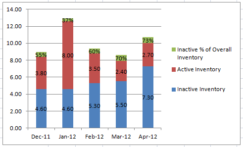
How To Show Percentages In Stacked Column Chart In Excel With a stacked column chart in Excel, you can view partial numbers, but what do you do when you want to show percentages?

Excel Chart Not Showing All Data Labels - Chart Walls
How to show percentage in Excel - Ablebits To apply the percent format to a given cell or several cells, select them all, and then click the Percent Style button in the Number group on the Home tab: Even a faster way is pressing the Ctrl + Shift + % shortcut (Excel will remind you of it every time you hover over the Percent Style button).
Excel Dashboard Templates How-to Put Percentage Labels on Top of a Stacked Column Chart - Excel ...
How to show percentage in pie chart in Excel? - ExtendOffice Show percentage in pie chart in Excel. Please do as follows to create a pie chart and show percentage in the pie slices. 1. Select the data you will create a pie chart based on, click Insert > Insert Pie or Doughnut Chart > Pie. See screenshot: 2. Then a pie chart is created. Right click the pie chart and select Add Data Labels from the context ...

How-to Use Data Labels from a Range in an Excel Chart - Excel Dashboard Templates
Data label in the graph not showing percentage option. only value ... Add columns with percentage and use "Values from cells" option to add it as data labels labels percent.xlsx 23 KB 0 Likes Reply Dipil replied to Sergei Baklan Sep 11 2021 08:47 AM @Sergei Baklan Thanks. It's a tedious process if I have to add helper columns. I have more than 100 such graphs in one excel. Thanks for your support.
33 How To Label Bar Graph In Excel
How to Show Percentages in Stacked Bar and Column Charts 1 – Select the range of cells you want to have this style of formatting. 2 – Click “New Rule” from the Conditional Formatting dropdown menu. 3 – Select “Format ...
Post a Comment for "41 how to show data labels as percentage in excel"