38 multiple data labels excel pie chart

Excel Chart VBA - 33 Examples For Mastering Charts in ... - Analysistabs We can create the chart using different methods in Excel VBA, following are the various Excel Chart VBA Examples and Tutorials to show you creating charts in Excel using VBA. 1. Adding New Chart for Selected Data using Sapes.AddChart Method in Excel VBA. The following Excel Chart VBA Examples works similarly when we select some data and click ... › comparison-chart-in-excelComparison Chart in Excel | Adding Multiple Series Under Same ... This window helps you modify the chart as it allows you to add the series (Y-Values) as well as Category labels (X-Axis) to configure the chart as per your need. Under Legend Entries ( S eries) inside the Select Data Source window, you need to select the sales values for the year 2018 and year 2019.

Best Excel chart to show percentage of total - Profit claims Just do the following steps: #1 select the original data to create a stacked column chart. #2 go to INSERT tab, click Insert Column Chart command under charts group, and select 2-D Column from the drop down list. #3 a stacked column chart has been created. #4 go to DESIGN tab, click Switch Row/Column command under Data group.

Multiple data labels excel pie chart

How to Apply a Filter to a Chart in Microsoft Excel - How-To Geek Select the data for your chart, not the chart itself. Go to the Home tab, click the Sort & Filter drop-down arrow in the ribbon, and choose "Filter." Click the arrow at the top of the column for the chart data you want to filter. Use the Filter section of the pop-up box to filter by color, condition, or value. › documents › excelHow to display leader lines in pie chart in Excel? - ExtendOffice To display leader lines in pie chart, you just need to check an option then drag the labels out. 1. Click at the chart, and right click to select Format Data Labels from context menu. 2. In the popping Format Data Labels dialog/pane, check Show Leader Lines in the Label Options section. See screenshot: 3. Close the dialog, now you can see some ... How to show all detailed data labels of pie chart - Power BI 1.I have entered some sample data to test for your problem like the picture below and create a Donut chart visual and add the related columns and switch on the "Detail labels" function. 2.Format the Label position from "Outside" to "Inside" and switch on the "Overflow Text" function, now you can see all the data label. Regards, Daniel He

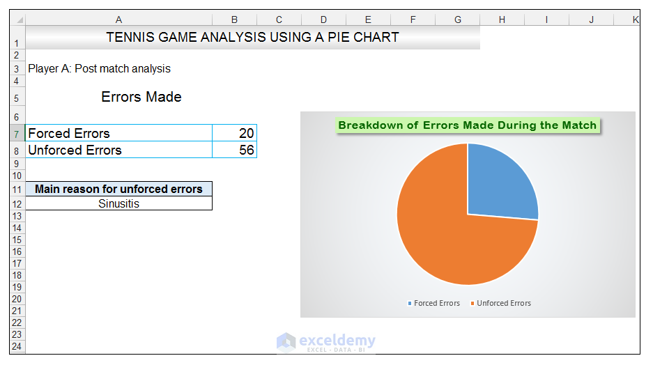
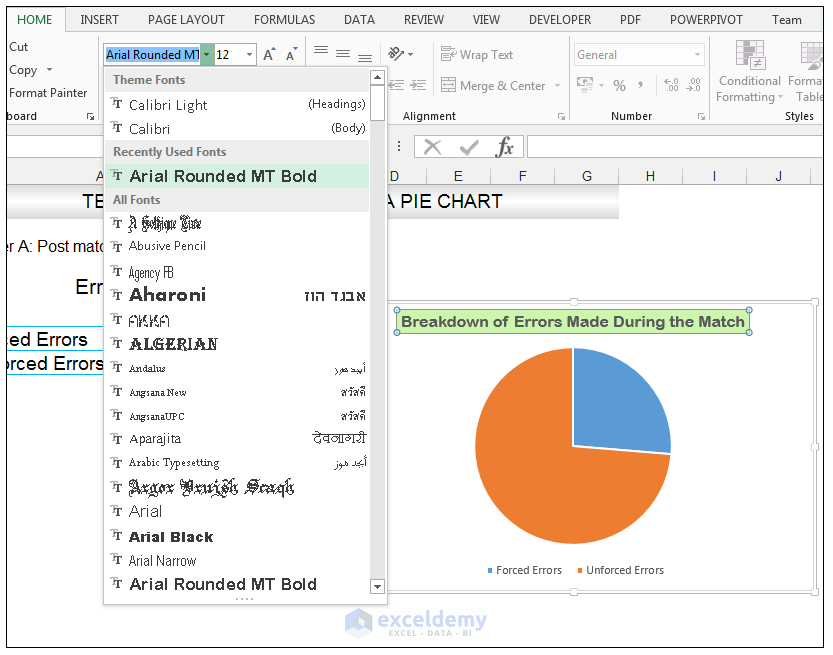
Multiple data labels excel pie chart. How to Make a Pie Chart in Excel - WinBuzzer Select your data, press the pie icon in the "Insert" tab of the ribbon, and click the pie of pie icon. A pie of pie chart in Excel is indicated by a picture of a big and small pie with lines ... › plot-multiple-data-sets-onPlot Multiple Data Sets on the Same Chart in Excel ... Jun 29, 2021 · You can further format the above chart by making it more interactive by changing the “Chart Styles”, adding suitable “Axis Titles”, “Chart Title”, “Data Labels”, changing the “Chart Type” etc. It can be done using the “+” button in the top right corner of the Excel chart. How to Create a Dynamic Pie Chart in Excel? - GeeksforGeeks It is the easiest method for creating a dynamic pie chart. So to this follow the following steps: Step 1: Create a table with proper headings and values inserted in it. Here, a table is created with Year-wise Sale, Tax, and Total (Sum of Sale and Tax) columns. Step 2: Copy the headings and paste them separately. How to Make a Pie Chart in Excel & Add Rich Data Labels to The Chart! Formatting the Data Labels of the Pie Chart. 1) In cell A11, type the following text, Main reason for unforced errors, and give the cell a light blue fill and a black border. 2) In cell A12, type the text Sinusitis, and give the cell a black border, and align the text to the center position. 3) Select the Unforced Errors data point only, (the ...

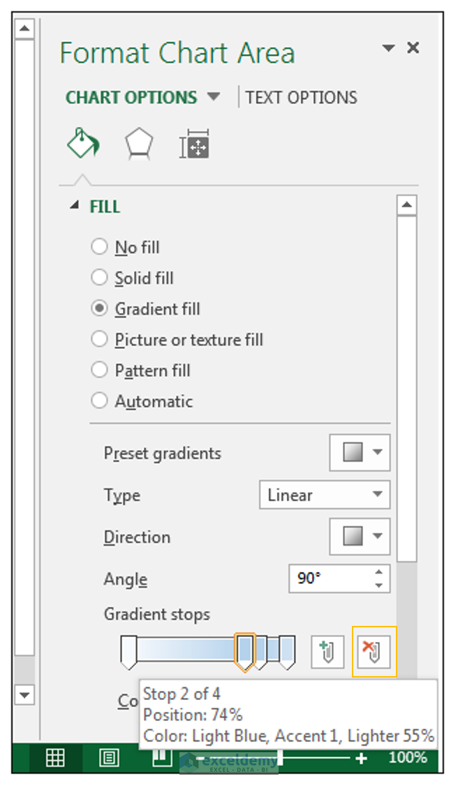
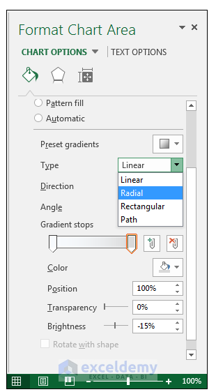
Pie Chart in Excel - Inserting, Formatting, Filters, Data Labels Right click on the Data Labels on the chart. Click on Format Data Labels option. Consequently, this will open up the Format Data Labels pane on the right of the excel worksheet. Mark the Category Name, Percentage and Legend Key. Also mark the labels position at Outside End. This is how the chark looks. Formatting the Chart Background, Chart Styles How to Create Pie Chart from Pandas DataFrame - Statology We can use the following syntax to create a pie chart that displays the portion of total points scored by each team: df. groupby ([' team ']). sum (). plot (kind=' pie ', y=' points ') Example 2: Create Custom Pie Chart. We can use the following arguments to customize the appearance of the pie chart: autopct: Display percentages in pie chart How to Add Leader Lines in Excel? - GeeksforGeeks Step 2: Go to Insert Tab and select Recommended Charts. A dialogue box name Insert Chart appears. Step 3: Click on All Charts and select Line. Click Ok. Step 4: A line chart is embedded in the worksheet. Step 5: Go to Chart Design Tab and select Add Chart Element . Step 6: Hover on the Data Labels option. Click on More Data Label Options …. Best Types of Charts in Excel for Data Analysis, Presentation and ... Learn to select best Excel Charts for Data Analysis, Presentation and Reporting within 15 minutes. ... Include percentages and labels for your pie chart to make it easy to read. ... 75% and 100%. Don't compare multiple pie charts. Do not use multiple pie charts for comparison as the slice sizes are really difficult to compare side by side.

How to Use Excel Pivot Table Label Filters - Contextures Excel Tips To change the Pivot Table option, and allow multiple filters, follow these steps: Right-click a cell in the pivot table, and click PivotTable Options. In the PivotTable Options dialog box, click the Totals & Filters tab. In the Filters section, add a check mark to 'Allow multiple filters per field.'. Click the OK button, to apply the setting ... How to Create Pie Charts in Excel: The Ultimate Guide - Classical Finance Adding labels to a pie chart is a great way to provide additional information about the data in the chart. To add click format data labels, select the pie chart and then go to the ribbon and click on the Add Data Labels button. This will add data labels for each pie chart slice that show the value of that data. How To Show Two Sets of Data on One Graph in Excel Choose "All Charts" and click "Combo" as the chart type From the options in the "Recommended Charts" section, select "All Charts" and when the new dialog box appears, choose "Combo" as the chart type. These let Excel know you want to work with multiple data sets before you even edit the graph. Create A Pie Chart From Excel Data - PieProNation.com How To Create A Pie Chart. Just like any chart, we can easily create a pie chart in Excel version 2013, 2010 or lower. First, we select the data we want to graph. Click Insert tab, Pie button then choose from the selection of pie chart types: Pie, Exploded Pie, Pie of pie, Bar of pie, or 3D pie chart. Figure 2.

How to Create Multi-Category Chart in Excel - Excel Board

Pie of Pie Chart in Excel - Inserting, Customizing - Excel Unlocked Customizing the Pie of Pie Chart in Excel Splitting the Parent Chart We can select what slices are going to be represented by the parent chart and subset chart. To begin:- Select the Chart. Go to Format Tab. Choose Series "Sales" in the Current Selection Group. Click on Format Selection Button. This would again open Format Series pane.

How to Represent Data with a Pie of Pie Chart in Your Excel Worksheet - Data Recovery Blog

A Step-By-Step Guide on How to Make a Pie Chart in Excel 3. Select your data values and create the chart. Highlight the data range by clicking on the cell on the top left corner and dragging it until you've selected all the cells with values you wish to include in the pie chart. Then go to the top left corner of your window and click the "Insert" tab next to the "Home" tab.

Creating Pie Chart and Adding/Formatting Data Labels (Excel) - YouTube

8 Types of Excel Charts and Graphs and When to Use Them - MUO Pie graphs are some of the best Excel chart types to use when you're starting out with categorized data. With that being said, however, pie charts are best used for one single data set that's broken down into categories. If you want to compare multiple data sets, it's best to stick with bar or column charts. 3.

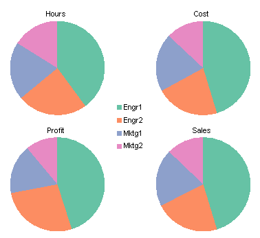
Column Chart to Replace Multiple Pie Charts - Peltier Tech Blog

How to Create a Bar Chart in Excel with Multiple Bars? To add data labels, go to the Chart Design ribbon, and from the Add Chart Element, options select Add Data Labels. Adding data labels will add an extra flair to your graph. You can compare the score more easily and come to a conclusion faster. You can also choose a column chart that will give you a similar result.

How to Make a Pie Chart in Excel & Add Rich Data Labels to The Chart!

› office-addins-blog › 2015/11/05How to create a chart in Excel from multiple sheets - Ablebits Nov 05, 2015 · Supposing you have a few worksheets with revenue data for different years and you want to make a chart based on those data to visualize the general trend. 1. Create a chart based on your first sheet. Open your first Excel worksheet, select the data you want to plot in the chart, go to the Insert tab > Charts group, and choose the chart type you ...

How to Represent Data with a Pie of Pie Chart in Your Excel Worksheet - Data Recovery Blog

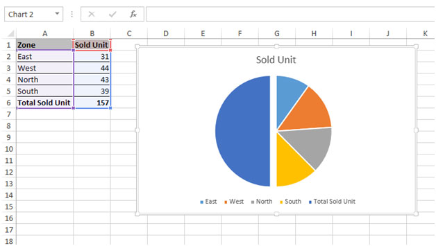
How to Make a Pie Chart with Multiple Data in Excel (2 Ways) - ExcelDemy First, to add Data Labels, click on the Plus sign as marked in the following picture. After that, check the box of Data Labels. At this stage, you will be able to see that all of your data has labels now. Next, right-click on any of the labels and select Format Data Labels. After that, a new dialogue box named Format Data Labels will pop up.

How to Make a Pie Chart in Excel Using Spreadsheet Data

Create Pie Chart In Excel - PieProNation.com Right click the pie chart again and select Format Data Labels from the right-clicking menu. 4. In the opening Format Data Labels pane, check the Percentage box and uncheck the Value box in the Label Options section. Then the percentages are shown in the pie chart as below screenshot shown.

Excel 2010 pie chart data labels in case of "Best Fit"

How to Make a Pie Chart in Microsoft Excel - How-To Geek While your data is selected, in Excel's ribbon at the top, click the "Insert" tab. In the "Insert" tab, from the "Charts" section, select the "Insert Pie or Doughnut Chart" option (it's shaped like a tiny pie chart). Various pie chart options will appear.

How to Make a Pie Chart in Excel & Add Rich Data Labels to The Chart!

Show data in a line, pie, or bar chart in canvas apps - Power Apps Add a pie chart Add a bar chart to display your data Use line charts, pie charts, and bar charts to display your data in a canvas app. When you work with charts, the data that you import should be structured based on these criteria: Each series should be in the first row. Labels should be in the leftmost column.

How to Make a Pie Chart in Excel & Add Rich Data Labels to The Chart!

How to set multiple series labels at once - Microsoft Tech Community Click anywhere in the chart. On the Chart Design tab of the ribbon, in the Data group, click Select Data. Click in the 'Chart data range' box. Select the range containing both the series names and the series values. Click OK. If this doesn't work, press Ctrl+Z to undo the change. Apr 09 2022 12:02 PM.

How to display leader lines in pie chart in Excel?

Display data point labels outside a pie chart in a paginated report ... Create a pie chart and display the data labels. Open the Properties pane. On the design surface, click on the pie itself to display the Category properties in the Properties pane. Expand the CustomAttributes node. A list of attributes for the pie chart is displayed. Set the PieLabelStyle property to Outside. Set the PieLineColor property to Black.

How to Make a Pie Chart in Excel & Add Rich Data Labels to The Chart!

› ms-excel-pie-chartHow to Make a Pie Chart in Excel (Only Guide You Need) Jul 13, 2022 · Read More: How to Make Pie Chart in Excel with Subcategories (2 Quick Methods) Conclusion. Hope after reading this article you will not face any difficulties with the pie chart. This article covers all the necessary things regarding Excel Pie Chart. Stay tuned for more useful articles. Let us know what problems do you face with Excel Pie Chart.

How to Make a Pie Chart in Excel & Add Rich Data Labels to The Chart!

How To Make a Pie Chart in Excel (With Tips) | Indeed.com First, right-click on the pie chart and select "Add data labels" to insert the numerical value of each piece onto the pie chart. If you want your pieces to show category names, you can edit them by right-clicking any label and selecting "Format data labels," followed by "Label options."

How to Make a Pie Chart in Microsoft Excel 2010 | Microsoft Excel Tips from Excel Tip .com ...

› pie-chart-examplesPie Chart Examples | Types of Pie Charts in Excel with Examples PIE Chart can be defined as a circular chart with multiple divisions in it, and each division represents some portion of a total circle or total value. Simply each circle represents the total value of 100 per cent, and each division contributes some per cent to the total.

How to Make Charts and Graphs in Excel | Smartsheet

spreadsheeto.com › pie-chartHow To Make A Pie Chart In Excel. - Spreadsheeto How To Make A Pie Chart In Excel. In Just 2 Minutes! Written by co-founder Kasper Langmann, Microsoft Office Specialist. The pie chart is one of the most commonly used charts in Excel. Why? Because it’s so useful 🙂. Pie charts can show a lot of information in a small amount of space. They primarily show how different values add up to a whole.

Share :